DPL Performance User Guide

Summary

As with any programmable, high-speed network processing component, NVIDIA Smart-NIC technology requires an awareness of the target capabilities to achieve the best performance. Tools such as the NVIDIA DOCA™ Pipeline Language (DPL) compiler use their knowledge of the platform and perform whole-program analysis to optimize your program as written, but the structural decisions you make as the programmer still influence the achievable performance. This guide provides the background information on NVIDIA networking platforms that you need to meet your application requirements.

This guide begins with a brief introduction to the device operation model: how packets traverse the processing pipeline and the operations performed on them. It then summarizes the principles that determine the performance a system achieves and gives examples of coding patterns that perform well. It ends with how to use compiler metric outputs together with on-device measurement to iterate on program adjustments.

Basic Device Model

DPL programs are primarily written to configure the packet processing pipeline, called the eSwitch in NVIDIA DPU and SuperNIC devices. This pipeline implements a common network processing paradigm called match-action. In a match-action pipeline, a packet logically traverses a sequence of tables, where the following two basic steps are performed:

1. Construct a match key based on packet contents, processing metadata, or both.

2. Use the match key to look up in a (hash) table which actions to perform, such as modifying the packet and directing it to its next destination.

The discussion that follows applies generally to most NVIDIA DPU and SuperNIC devices, though it was written for an NVIDIA BlueField-3 device.

Figure 1 shows an example of a 3-stage program, in which a packet progresses from left to right. In the first match-action stage, Key 1 is constructed from the contents of the packet. Key 1 is then used to look up Table 1, which finds entry E1. Entry E1 indicates to perform Actions 1, which might modify the packet or perform some other operation. The packet then progresses to the next match-action stage, where similar operations are performed: Key 2 is constructed to look up Table 2, which finds entry E2 that indicates to perform Actions 2. In the final stage of this example, the packet goes through similar operations a third time.

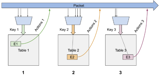
Figure 1: Simple 3-stage Match-action Pipeline.

NVIDIA networking devices perform these match-action steps using custom hardware components, which allows high-throughput, low-latency processing. To fully optimize a DPL program, you need to understand how these basic hardware components are structured. The rest of this section describes the basic building blocks of the hardware.

Packet Parsing and Accessible Fields

The hardware has a dedicated packet parsing engine that understands a wide range of standard protocols and encapsulation formats. This fixed parsing engine can also be extended to support transitions to and from custom header formats, and to extract that custom header data for use in the match-action pipeline. Custom header formats can add processing time, because additional packet data is examined.

The packet parsing engine’s primary task is to populate a large header structure with packet header data and parsing metadata, such as validity bits for headers and convenient type information (for example, L3 type or L4 type). The match-action pipeline can use the header structure to form match keys, and can read or write it as part of action processing.

Because actions can change the encapsulation of a packet, the packet parsing engine might run again after each match-action stage to update the header structure. This reparsing incurs a slight processing cost, because the packet data must be reexamined. As a result, each match-action stage sees the most up-to-date packet header data.

In general, packet header data is accessible from the header structure at the granularity of packet header fields. However, the hardware generally operates on units of bytes or DWORDs (4 bytes). This means that packet header fields larger than 4 bytes are logically split into more than one access. Packet header fields smaller than a byte remain a single access, but they might be packed with other small fields to optimize storage space. The DPL compiler is aware of this fixed header structure and optimizes match key creation, packet field access, or both to account for it.

Because of hardware constraints, not all data in the header structure can be used in the same way. For example, some packet header fields can’t be used to form a match key, and some can’t be used in assignment operations. These restrictions are summarized in the DOCA Target Architecture document.

Key Construction

A table key is constructed by concatenating relevant packet fields, metadata fields, or both, reading one or more bytes from the header structure. The hardware block that constructs keys must read from the header structure at byte granularity, so the final constructed size is at least the sum of the sizes of the individual key fields. For example, Figure 2 shows how a table key that is notionally 3 bytes long actually consumes 4 bytes at the hardware level, because two of the small key fields occupy different bytes in the header structure. The hardware applies a mask to clear any unused bits from the bytes that it reads from the header structure.

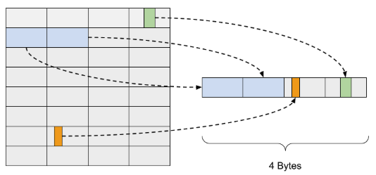
Figure 2: Match keys are formed by reading one or more bytes from a hardware header structure.

The hardware block that constructs a match key has some limits, summarized in Table 1, that depend on the type of matching operation. The hardware has a maximum amount of data it can read at different granularities. For a single exact match operation, the maximum size of the hardware key that can be formed is 44 bytes. For a single range match lookup, the maximum formed key size is 16 bytes, though the lookup operation limits that to at most four fields of up to 4 bytes each. Large keys affect whether actions can be packed in the table entry, as described in more detail in the Action Processing section.

Table 1: Match Key Construction Limits.

Tables and Table Lookup

After a match key is formed, a lookup operation is performed in a table allocated in memory. The hardware supports two primary forms of tables: hash tables and range tables.

Hash Tables

In a hash table, a hash value is computed on the constructed match key. The hash value provides a hash bucket address, which is essentially the head pointer for a linked list. The lookup operation fetches the head entry and compares the match key values to those stored in the entry. If they match, the entry matches, and the hardware executes the actions associated with the entry. If they don’t match, the next element in the "linked list," if any, is fetched and compared in the same way. If no match is found after the full list is searched, the entry misses, and the table’s default action is executed. This hardware linked-list structure is how hash collisions are resolved.

Figure 3 shows an example of how the hardware walks through a particular hash bucket to find the correct entry. First, a match key is formed, with values that correspond to a GREEN entry. Second, a hash calculation on the formed match key produces the result h. The hardware fetches the memory address associated with address h and compares the head entry to the match value. Because the first entry (RED) doesn’t match, the hardware fetches the next entry at hash bucket h (PURPLE). This entry doesn’t match either, so the next entry (GREEN) is fetched. The GREEN entry matches, so the actions associated with the entry are performed.

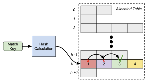
Figure 3: Hash Lookup Table with Hash Collision Resolution.

Resolving hash collisions can degrade performance, because each entry that is examined incurs an additional memory access. In most use cases, especially for large tables, the entries aren’t known in advance, so a perfect hash function with no collisions isn’t feasible. However, one trade-off to consider for reducing the likelihood of hash collisions is to allocate more space for the table by increasing its size. This increases the number of available hash buckets that the hash calculation can address. This trade-off is described in more detail in the Reducing Hash Collisions section.

A table miss isn’t a free operation. In Figure 3, if the match key hashes to location h − 1, where there is no entry, the hardware still performs a memory access at that location to confirm that there’s no matching entry. If there are default actions to perform, the miss address directs the packet flow to an always hit default entry table to perform the default actions. In a more complex case, if the match key hashes to location h in Figure 3, but entries 1, 2, 3, and 4 all don’t match, four memory accesses are performed before the hardware determines that the table missed. Depending on the default actions to perform, the packet flow might go to an always hit default entry table.

Range Tables

A range table differs from an exact match (hash) table in that, for certain keys, the values that make an entry match can fall within an inclusive interval between a minimum and a maximum. For example, if you range match on the TCP source port, you can provide an entry that says source ports between 50 and 100, inclusive, match the entry.

Because of the way the DPU hardware progresses through processing, a range match table generally can’t contain only keys that perform range matching; you must also specify at least one exact match key. The hardware needs a fast way to narrow down the set of entries to examine, because a linear search of all entries in a large range table isn’t feasible. As a result, a range table consists of two parts, as shown in Figure 4.

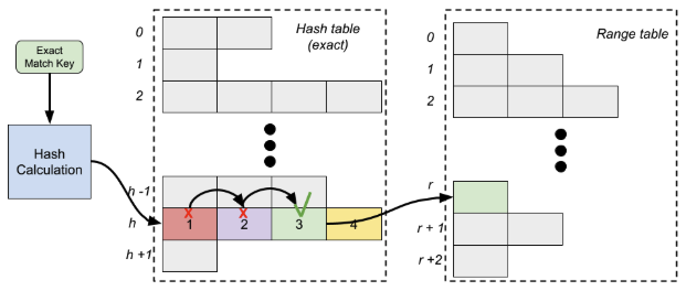
Figure 4: Example Range Match Table.

The first part handles exact match keys using the normal hashing mechanism described earlier. However, after any collisions are resolved and an entry that matches the exact match portion is found, the hardware proceeds to a range table instead of performing the entry’s actions. In this second-part range table, the range keys are handled by comparing the current packet’s value for each key against the interval indicated for that entry. If each range key’s value is within the interval between its minimum and maximum values, the overall entry matches, and the entry’s actions are performed. Because multiple logical table entries can share the same exact match subset of an entry, the hardware might inspect more than one range table entry to determine whether the overall entry matches.

A single range table can perform at most four 32-bit range match operations, which translates to at most four range match keys, regardless of key width. For example, range matching on both the TCP source and destination ports uses two of the 32-bit range match operations, even though each port field is only 16 bits.

Action Processing

A table lookup results in either a table hit, meaning a matching entry was found, or a table miss, meaning no matching entry was found. Regardless of the lookup outcome, the next phase in the match-action paradigm is action processing.

Action processing is a generic term, but on NVIDIA networking devices, it refers to six types of operations:

• Packet header field or metadata modification: Actions that change the value of one or more packet header or metadata fields, such as decrementing a TTL, assigning an IP address, assigning an L4 port, or assigning a packet field to be the result of a hash calculation.

• Packet structural changes: Actions that modify the structure of a packet by adding or removing bytes, as is typical in packet encapsulation or decapsulation. Packet structural changes generally require rerunning the parser to repopulate the header structure.

• Cloning: Actions that copy a packet for multicast operations, to send the packet to the control plane for further processing, or both.

• Stateful flow-based operations: Actions that maintain state based on packet flows, such as counters for statistics, metering operations that help inform a forward or drop decision, and entry aging.

• Encryption: Actions that encrypt or decrypt the packet payload.

• Updating the control flow: Actions that direct the packet to its next destination, such as applying a next table, forwarding the packet to an interface, or dropping the packet.

Action "instructions" are stored alongside the match values in the table entries described in the previous section. Table entries have a fixed size, so there is a limit to how many actions a single table entry can initiate. The match key size affects how many actions can be stored in the table entry. When a complex DPL action requires more hardware actions than fit in a single table entry, the hardware can chain multiple table entries together, as shown in Figure 5. The first table entry in the action chain resolves whether the logical entry matches, and the subsequent table entries are advanced to directly and are configured to "always match," so their stored actions are executed.

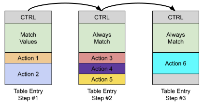
Figure 5: Chaining table entries to hardware actions.

Each step in the chain incurs a memory access that fetches a relevant table entry. Complex action chains require more processing time because of the additional steps needed to complete them. There isn’t a one-to-one correspondence between DPL action statements (such as nv_set_l4_src_port(param)) and hardware actions. The hardware has dedicated logic components that execute actions, which allows multiple primitive operations to be executed in parallel or in quick succession.

Guiding Principles for Performance

The primary influence on overall performance (that is, latency and throughput) is the number of table entries that must be fetched from memory and processed for each packet that enters the system. Each match-action step is called a hop. To achieve the best performance for any given processing path, reduce the number of hops.

Hardware hops come from the following sources:

• Each logical table incurs at least one hop to resolve its match operation and perform actions.

• A logical table that performs range matching requires at least two hops to resolve the match operation and perform the actions.

• A logical table that performs non-equality comparisons (for example, field1 < field2) requires at least two hops to resolve the match operation and perform the actions.

• A logical table that performs longest prefix match (LPM) matching, ternary matching, or both requires a tree of lookups and therefore additional hops.

• The hardware has an allocation limitation on single objects. Very large tables require a three-hop implementation: calculating a hash index, selecting a shard table, and looking up the entry in the sharded table.

• Each hash collision in a logical table incurs at least one hop, because an additional table entry (memory location) must be processed to resolve the collision.

• Complex actions that require an action chain of table entries require an additional C hops, where C is the length of the action chain after the match operation.

A secondary influence, though related to the first, is the performance of the memory subsystem cache. When table entries and associated resources reside in cache, the processing time associated with a hop is reduced. Ideally, all table entries associated with an application reside in cache. In practice, table scale makes this impossible because of the limited size of the cache.

Allocated memory is also a performance consideration, because deployed devices don’t have unlimited memory. Memory consumption is directly proportional to the complexity of the DPL program, in terms of the number of tables, table sizes, action complexity, and necessary control branching.

Reducing Hops on Critical Paths

Although the DPL compiler performs many optimizations that restructure a DPL program for an efficient implementation, its analysis is limited to compile-time information. Analysis based on expected use cases, critical program paths, and runtime-added table entries requires the application developer’s knowledge.

In most cases, a DPL program frequently executes only a subset of the many potential processing paths a packet can take. For example, core processing is more likely to be executed than error handling. These frequently exercised processing paths are called critical paths. Optimizing them has more potential for performance gains than optimizing less frequently used paths.

As described in the DPL Compiler Outputs section, the compiler reports the worst-case path found in the program in terms of the number of hops and maximum processing cost, but this path doesn’t necessarily coincide with a critical path.

As the DPL program author, you should profile your program using domain knowledge, application specifications, and measurement (described in the Measurement section) to identify critical paths. The match-action steps along these paths become candidates for restructuring, simplification, or both, using techniques such as the following:

• Combining tables to reduce the number of lookups

• Collapsing control branching conditional tests into existing table lookups

• Using metadata to defer common, non-terminal action execution

• Distributing complex actions across existing tables

• Removing action dependencies to allow tighter packing

Combining Tables

Reducing the number of lookups reduces the number of hops, and one way to do this is to combine tables. The DPL compiler can’t generically combine dynamic tables (tables with runtime-added entries), because doing so affects the control plane interface.

For example, a DPL program that applies two exact match tables in sequence might be a candidate for combining. You can combine the tables by merging the table keys, expanding the actions, and (likely) adjusting the table size.

table table1 {
       key = {
           headers.vlan.vlan_id : exact;
       }
       actions = { action1a; action1b; }
       size = 4096;
   }


   table table2 {
       key = {
           headers.ipv4.ttl : exact;
       }
       actions = { drop; forward; }
       size = 16;
   }
   apply {
       table1.apply();
       table2.apply();
   }

The following example shows the transformed program. The table keys are merged so that the combined table matches on both vlan_id and ttl. The actions are amended to provide the cross product of the behavior, so there are two variants of action1a: one that includes the drop behavior, and one that includes the forward behavior. Finally, knowledge of the expected table entries in table2 shows that the application cares about ttl values of 0 and 1 for determining whether to use drop. This information is used to set the combined table size to 16384.

table table_combined {
       key = {
           headers.vlan.vlan_id : exact;
           headers.ipv4.ttl : exact;
       }
       actions = { 
           action1a_and_drop;
           action1a_and_forward;
           action1b_and_drop;
           action1b_and_forward;
       }
       size = 16384;
   }
   apply {
       table_combined.apply();
   }

In this case, the design trades more overall memory consumption for fewer lookups. Combining tables that use additional resources needs extra consideration, especially when those resources must scale with the number of table entries, such as direct counters or direct meters. Packet modifications that assign a runtime value (for example, an action parameter) to packet or metadata fields also use extra memory to store the action parameter values, which results in additional memory allocation.

Collapsing Control Branching

As with combining tables, you can combine control flow branching expressions into dynamic tables. The hardware implementation of a conditional statement requires a lookup. For example, the following DPL program snippet requires two lookups:

table table1 {
       key = {
           headers.vlan.vlan_id : exact;
       }
       actions = { action1a; action1b; }
       size = 4096;
   }
   apply {
       if (std_meta.vlan_type == VLAN_TYPE_SVLAN) {
           table1.apply();
       }
   }

If you bring the condition into the table, you can eliminate a hop by eliminating the conditional test match step. Because the original program applies table1 only when vlan_type is VLAN_TYPE_SVLAN, you can augment all runtime entries to require that value. In this case, no additional entries or memory are required.

table table_combined {
       key = {
           headers.vlan.vlan_id : exact;
           std_meta.vlan_type : exact;
       }
       actions = { action1a; action1b; }
       size = 4096;
   }
   apply {
       table_combined.apply();
   }

Removing Action Dependencies

Complex actions might require implementation through an action chain, where each step in the chain is a hop in the hardware. Although the hardware can execute some actions in parallel, the compiler can’t configure it to do so if there are dependencies between actions (for example, write after read or read after write). Dependencies prevent the compiler from packing actions together, which can lead to longer action chains.

Distributing Complex Actions

Tables that execute complex actions might require multiple hops to execute all of the action’s requirements. The DPL compiler must place actions in an action chain for the following reasons:

• Hardware packing limitations: Table entries have a fixed size, so there’s a maximum number of actions allowed per table entry.

• Action dependencies: As described earlier, action dependencies might force the DPL compiler to move part of an action to a separate table entry so that the dependency can be resolved.

Depending on the DPL program’s deployment scenario, you might be able to distribute subsets of actions into the actions of other tables that are known to execute in the same scenario.

For example, consider a packet processing path through three tables, as shown in Figure 6, where the packet proceeds through Table 1 executing action A1; Table 2 executing actions B1, B2, B3, B4, and B5; and Table 3 executing action C1. In this case, Table 1 has no action chain (1 hop), Table 2 has an action chain of length two (3 hops total), and Table 3 has no action chain (1 hop). If a DPL developer knows that actions B3 and B5 are always executed on this path, those actions can be distributed into the surrounding tables to improve the packing. If the DPL developer further knows that action B5 has a dependency on action B4, then action B4 isn’t a candidate to move later.

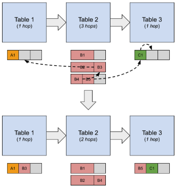
Figure 6: Example of Distributing Actions.

The second half of Figure 6 shows how moving the actions reduces the overall hop count by 1, because the action chain of Table 2 is reduced by 1.

Deferring Actions

When multiple tables have complex action chains, introducing an additional lookup table with an action built from parts of previous actions can sometimes reduce the overall hop count. Consider the example in Figure 7, which executes three tables in sequence: Table 1 with actions A1, A2, A3, and A4; Table 2 with actions B1, B2, B3, and B4; and Table 3 with actions C1, C2, and C3. Because of packing constraints, dependencies, or both, each of these tables requires an action chain, for a total of 8 hops.

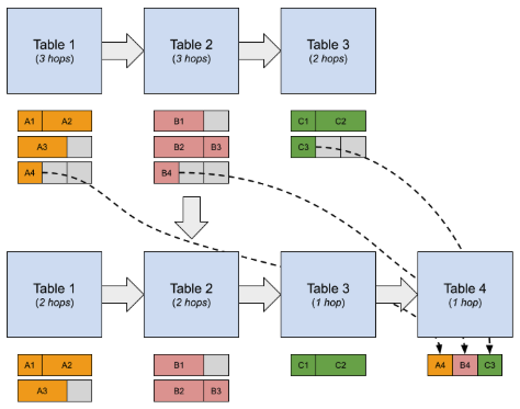
Figure 7: Example of Deferring Actions to a New Table.

If the DPL developer recognizes that actions A4, B4, and C3 can be executed later, it might be beneficial to introduce an additional lookup table that executes these actions in a deferred manner. The declaration for Table 4 could look like the following code snippet. The program carries a metadata bit for each action that indicates whether to run that action, and Table 4 uses these bits as match keys. There are 8 varieties of actions to run in Table 4, corresponding to the 8 possibilities for the metadata values.

table table4 {
       key = {
           user_meta.run_a4 : exact;
           user_meta.run_b4 : exact;
           user_meta.run_c3 : exact;
       }
       actions = { 
           run_a4;
           run_a4_b4;
           run_a4_c3;
           run_a4_c3;
           run_b4;
           run_b4_c3;
           run_c3;
           run_a4_b4_c3;
       }
       size = 8;
   }
   apply {
       table4.apply();
   }

With this approach, the overall hop count is reduced to 6, even though a table was added.

Count Action

The COUNT action is a special-case action in the hardware, because it has a dedicated location in a table entry and is executed before any other actions in the table entry. As a result, packet length changes from other actions in the table entry (that is, reformatting actions) aren’t considered for the COUNT operation. This behavior causes a dependency that the compiler handles. For example, consider the following two actions.

action uses_one_hop(bit<32> index) {
    my_counter.count(index);
    nv_pop_headers(
        headers,
        NvAnchor.IP_START_OF_HEADER,
        NvAnchor.L4_START_OF_HEADER,
        /* do_updates */ false,
        /* do_reparse */ true);
}

action uses_two_hops(bit<32> index) {
    nv_pop_headers(
        headers,
        NvAnchor.IP_START_OF_HEADER,
        NvAnchor.L4_START_OF_HEADER,
        /* do_updates */ false,
        /* do_reparse */ true);
    my_counter.count(index);
}

Semantically, the count operation in the uses_one_hop action must occur before the nv_pop_headers reformatting operation. As a result, these two operations can be packed into one table entry. However, the second action, uses_two_hops, has a different semantic meaning. The count operation happens after the nv_pop_headers operation, meaning that the packet byte count adjustment should reflect the packet length change that results from nv_pop_headers. This dependency causes the two operations to be placed in two different table entries.

Ordering if/else Conditions by Likelihood

Conditional control flow branches (that is, if / else if / else chains) are implemented as a sequence of table lookups. To reduce the expected number of hops for any given packet, you should order these chains from most likely to least likely, as shown in Figure 8.

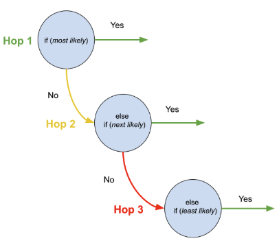
Figure 8: Conditional control flow branching is implemented as a sequence of table lookups.

Putting the condition most likely to be true first avoids additional lookups to resolve the control flow branching.

The preceding discussion assumes that the conditions are dissimilar. If the conditions test equality of fields against different values, the compiler can collapse the chain into a single table lookup. For example, the compiler collapses the following conditional tests into a single table lookup, where the table has multiple entries that dispatch to different paths.

apply {
    if (headers.ipv4.src_addr == 32w0x11110011) {
        ...
    } else if (headers.ipv4.src_addr == 32w0x11110022) {
        ...
    } else if (headers.ipv4.src_addr == 32w0x11110033) {
        ...
    } else {
        ...
    }
}

Squashing Conditions

The compiler performs static analysis of conditional branch chains and any nested conditional branches to try to automatically merge the conditions into a single (ideally) dispatch table, similar to how conditions were collapsed into a table in Collapsing Control Branching. This optimization lets you write a more readable set of logical conditions without sacrificing performance.

The DPL compiler tries to balance competing considerations: final match key size, total memory usage, and total number of hops. The optimization isn’t applied if the merged conditions need more than 6 hardware match keys or if the resulting merged table requires more than 128 entries.

Reducing Hash Collisions

Resolving hash collisions incurs additional hops in the hardware, so reducing collisions generally helps increase performance.

The hash function used by the hardware is fixed, but the DPL compiler can permute how the key data is provided to the hash generator. The DPL compiler uses this capability for static-entry tables to reduce and, in many cases, eliminate hash collisions. However, for dynamic-entry tables, where the entries are unknown at compile time, the compiler can perform only limited analysis.

As a DPL application developer, you can improve hashing performance for dynamic-entry tables in the following ways:

• Change the table size.

• Experiment with the nv_high_entropy_bits match key annotation.

Table Size

Adjusting the table size is the most direct way to try to reduce hash collisions, at the expense of increased memory consumption. Increasing the table size can reduce the likelihood of a hash collision, because there are more hash buckets where an entry can be placed, as shown in Figure 9.

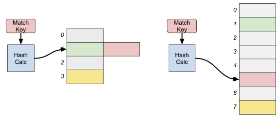
Figure 9: Hash Collision Avoidance by Increasing Table Size.

High Entropy Bits

Hashing performance depends on the inserted table entries, which aren’t known at compile time for dynamic-entry tables. To give the DPL compiler information about which match keys are important for hashing performance, you can add an annotation called nv_high_entropy_bits to one or more exact match keys. The DPL compiler uses this annotation to optimize how the match key is constructed.

The nv_high_entropy_bits annotation indicates which bit or bits of the annotated match key are expected to vary most across the table entries. The DPL compiler uses this information to place those bits in the locations that have the most impact on hashing performance.

table table1 {
       key = {
           headers.ipv4.src_addr : exact @nv_high_entropy_bits(0x7);
           headers.ipv4.dst_addr : exact @nv_high_entropy_bits(0xE00);
           headers.ipv4.protocol : exact;
           headers.tcp.src_port : exact;
           headers.tcp.dst_port : exact;
       }
       actions = { ... }
       size = 65536;
   }

In this example 5-tuple lookup, the annotations indicate that the three least significant bits of ipv4.src_addr and bits 17 to 19 of ipv4.dst_addr are expected to be high entropy. Knowing which bits to set requires some iteration and measurement with inserted table entries. You can gather this information, for example, by profiling the entries you expect to add and understanding a particular deployment scenario.

Optimizing for Cache Access

The hardware’s implementation of the match-action paradigm compares packet values against table entries stored in memory. Each hop requires at least one memory access to fetch a table entry’s match values and the actions to perform. Aggregate performance is much better when the accessed memory locations remain in the system cache. Because cache is a limited resource and fitting an entire DPL application in cache generally isn’t feasible, this section focuses on keeping critical path processing in cache.

Counterintuitively, in some situations, introducing additional hops performs better if the restructured program flow can remain in cache. For example, instead of one large table with equally likely entries, three smaller hierarchical tables that can remain in cache might perform better, as shown in Figure 10.

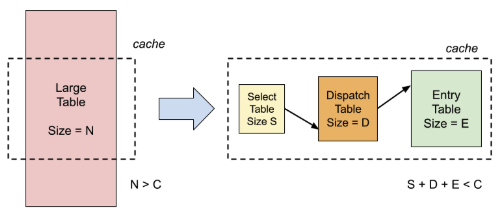
Figure 10: Restructuring large tables into smaller hierarchical tables might improve cache performance.

DPL Compiler Outputs

As described in the DPL Program Metrics document, the DPL compiler outputs a program_name.metrics.log file to the output build directory. Metrics output is enabled by default, which is equivalent to including the --enable metrics compile option.

The metrics report contains three main sections:

• Table of per-matcher and per-rule resource and processing costs

• Worst-case path identification, in terms of worst-case hop count and worst-case packet processing cost

• Static-entry table hash performance analysis (included only when the program uses static-entry tables)

You can use this information as a guide to help develop a DPL program and to identify potential performance bottlenecks.

Measurement

When possible, it helps to have a test environment with a development platform in which you can measure performance. Figure 11 shows an example setup.

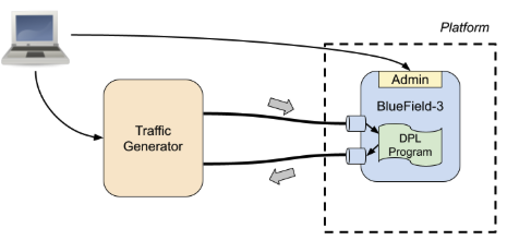
Figure 11: Example Measurement Test Environment.

In such a setup, you can iterate on DPL program modifications, load the program into a real device, add entries, and configure a network traffic generator to send and receive test packets or packet streams. The traffic generator can provide test results in terms of measured latency and maximum packet rates. With a setup like the one in Figure 11, you can modify a DPL program and obtain new measurements to confirm that structural changes provide the intended results.

Last updated: October 29, 2026